What is the Relationship between Shot Percentage and Wins?

In this Edition

• Breaking Down the Question
• Why is Shot Percentage Important?
• Modeling the Relationship between Shot Percentage and Wins
• Running a Correlation Analysis

Breaking Down the Question

The question here looks straightforward, so let's try and break it down: What is the Relationship between Shot Percentage and Wins?

From the question, we can derive three items:

• What is the nature of the measurement
• the Relationship reflects the statistical strength or weakness of how shot percentage impacts wins
• between Shot Percentage and Wins are the two variables between which we're measuring the relationship

While breaking down the question is straightforward, you'll need to figure out the best approach to model the relationship between shot percentage and wins.

Let's explore shot percentage as a metric first, and then, we'll move to modeling the relationship

Why is Shot Percentage Important

Shot percentage, also known as shooting percentage, is a hockey statistic that measures a team's efficiency at converting their shots on goal into actual goals. It's a simple concept: the higher the shot percentage, the more proficient a team is at capitalizing on their scoring opportunities. In the words of Wayne Gretzky, "You miss 100% of the shots you don't take," so shots are critical to scoring and so critical to winning.

Analysts calculate the shot percentage by dividing the number of goals scored by the total number of shots on goal. The formula looks like this:

Shot Percentage (%) = (Goals Scored / Total Shots on Goal) * 100

Beyond deriving a calculated perspective on the effectiveness of a team's (or player's) shots on goal, below are examples of the information shot percentage provides:

• Offensive Efficiency Evaluation: Shot percentage serves as a barometer of a team's offensive prowess. A high shot percentage indicates that a team is making the most of its scoring chances, showcasing the proficiency of its forwards and the quality of its offensive strategies.
• Goalie Assessment: Conversely, for goaltenders, shot percentage can be an essential tool for self-evaluation. A goalie's ability to stop high-percentage shots is a significant factor in their overall performance. Analyzing shot percentage against a specific goalie can reveal their strengths and weaknesses.
• Game Strategy Adjustments: Teams can use shot percentage data to fine-tune their game strategies. For instance, if a team's shot percentage is low, they may need to work on creating higher-quality scoring opportunities, while a high shot percentage might prompt them to continue their current tactics.

While shot percentage offers valuable insights, we must also recognize its limitations. It's a snapshot of a team's offensive efficiency — it doesn't tell the whole story. Here are some aspects that shot percentage doesn't capture:

• Defensive Performance: Shot percentage focuses exclusively on offensive efficiency and doesn't account for a team's defensive capabilities. A team might have a high shot percentage and struggle defensively, leading to losses.
• Quantity vs. Quality: Shot percentage doesn't distinguish between low-quality and high-quality shots. A team might have a high shot percentage but rely on low-percentage shots, which isn't a sustainable strategy.
• Score Effects: Teams with a comfortable lead may exhibit lower shot percentages because they prioritize defense over offense. Conversely, teams trailing may take riskier shots to catch up, affecting their shot percentage.

Modeling the Relationship between Shot Percentage and Wins

While a higher shot percentage generally correlates with more wins, several factors influence this connection. Here are three ways to model and analyze the relationship between shot percentage and wins:

• Correlation Analysis: Correlation analysis assesses the statistical relationship between shot percentage and wins. Data from multiple seasons or teams can be used to calculate a correlation coefficient (usually Pearson's r) that quantifies the strength and direction of the relationship. A positive correlation suggests that as shot percentage increases, so do wins.
• Regression Modeling: Regression analysis takes the relationship further by modeling wins as a function of shot percentage while controlling for other variables. This allows analysts to identify how much of a team's success can be attributed to shot percentage, accounting for factors like goals against, power-play efficiency, and penalty kill effectiveness.
• Predictive Modeling: Predictive modeling extends the analysis to forecast future performance. Analysts can build predictive models that use shot percentage as a predictor variable to estimate the number of wins a team is likely to achieve in an upcoming season. Machine learning algorithms, such as linear regression or random forests, can be valuable tools in this process.

Depending on how you want to model the relationship between shot percentage and wins, you will need data sets that may include game-level and/or season-level variables. Here's a list of useful data elements:

• Team-level statistics: Goals scored, total shots on goal, goals against, power-play percentage, penalty kill percentage, and more.
• Game-level data: Individual game results, including wins and losses.
• Player-level statistics: Player performance metrics, such as goals, assists, and time on ice, can help assess the impact of individual players on shot percentage.
• Advanced metrics: Additional advanced statistics, like expected goals (xG) and Corsi, can provide deeper insights into shot quality and possession.
• Historical data: Data from multiple seasons to conduct longitudinal analyses and assess trends over time.

Let's put some of the above into practice by collecting multiple seasons' worth of team data and building 1) a regression model and 2) a correlation analysis.

Running the Analyses

To build a regression model and conduct the correlation analysis, we collected five seasons worth of team data. We use My Sports Feeds as our data provider, but you can source and combine team statistics data from Hockey-Reference or another data source of choice.

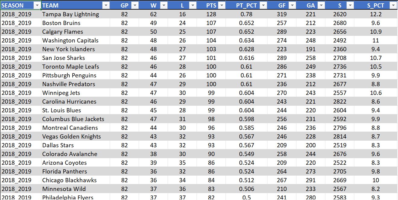
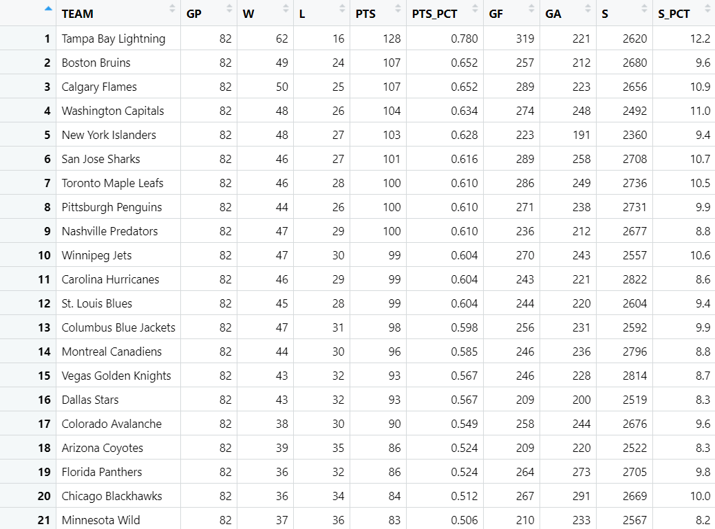
In our dataset, we have the following data elements for five regular seasons worth of NHL team data:

• Season (SEASON)
• NHL Team (TEAM)
• Games Played (GP)
• Wins (W)
• Losses (L)
• Points (PTS)
• Points Percentage (PT_PCT)
• Goals For (GF)
• Goals Against (GA)
• Shots (S)
• Shot Percentage (S_PCT)

Generally, it’s good to have more data elements than you need, so you can evaluate other relationships between other variables in your dataset and wins. Below is a snapshot of a curated Excel spreadsheet showing a subset of the multi-season team data.

Regression Model

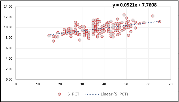
With the data in Excel, you can now create a linear regression between shot percentage (S_PCT) and wins (W). This line will indicate whether there is a positive (slopes up and to the right) or negative (slopes down and to the right) and the steepness of the slope represents the strength of the linear model.

To create a linear regression in Excel:

• Select the W and S_PCT columns.
• Click Insert, Recommended Charts, All Charts, and select the X Y (Scatter) chart.
• Click the "+" sign (Chart Elements) to the right of the scatterplot and check the Trendline.
• Right-click the trendline and click Format Trendline.
• In the Format Trendline pane, select Display Equation on the chart.

Format the chart to your liking — it should look similar to the one below. Now this is a simple linear regression, but it does give you some information about the strength of the relationship. And while the slope of the regression is up and to the right, it is not strong.

You can get a more detailed linear regression in Excel. To do this:

• Make sure the Data Analysis Tools are installed. (For more information on how to do this, go here.)
• Click Data Analysis, Regression, and OK.

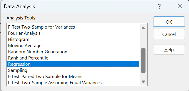
• Select the W column for your dependent variable (which is the Y axis), and select S_PCT for your independent variable (which is the X axis).
• The result should be similar to the spreadsheet below.

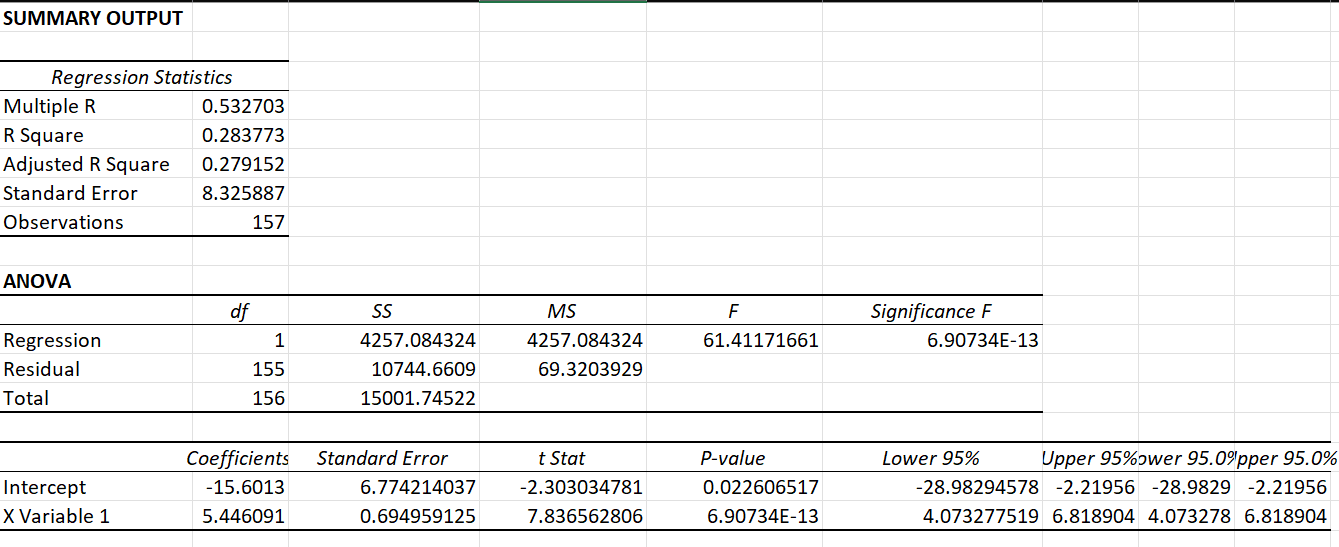
The results calculate and show how well the linear regression equation fits with the multi-season team stats data. We won't go into all of the numbers but will call out the Multiple R coefficient —  which runs from -1 to 1. Here we see this coefficient is 0.52, which is not very strong. (A number indicating a stronger relationship would be 0.70 or above.)

Our conclusion from this would be that while shot percentage seems to impact wins, there are other factors that influence the win as well. And logically, this makes sense; there are many different aspects that contribute to a win.

Correlation Analysis

While linear regression shows the strength of variables with one another, by using a correlation analysis, we can see how multiple variables correlate with one another. This type of analysis is typically the beginning point of a hockey analysis — to see where the strength lies in relationships across variables.

For this analysis, we'll use R and RStudio. Note that the dataset remains the same source file; however, we'll be analyzing that same data in a different way.

We’ve created two code snippets to illustrate how to create the correlation analysis.

The first code snippet shows how you read in the team stats data from the CSV file and then create a data frame that is a subset of the original dataset (sub_team_stats_df).

multi_year_team_stats_df <- read.csv("Combined_Team_Stats.csv")

sub_team_stats_df <- subset(multi_year_team_stats_df, select = 
    c("Team", "GP", "W", "L", "PTS", "PTS.","GF", "GA", "S", "S."))

colnames(sub_team_stats_df) <- c("TEAM", "GP", "W", "L", "PTS", "PTS_PCT", 
                                 "GF", "GA", "S", "S_PCT")

The result of the above is the following data frame.

The second code snippet subsets the earlier data frame, which then creates a correlation matrix using this data. The result of this is a correlation plot that shows the relative strength across variables.

library(ggcorrplot)
library(ggthemes)

cor_sub_team_stats_df <- subset(sub_team_stats_df, select = 
    c("GP", "W", "L", "PTS", "PTS_PCT", "GF", "GA", "S", "S_PCT"))

cor_matrix <- cor(cor_sub_team_stats_df)

ggcorrplot(cor_matrix, hc.order = TRUE, type = "lower", lab = TRUE,
           outline.color = "gray",
           colors = c("#6D9EC1", "#FFFFFF", "#E46726")) + 
  ggtitle("Correlation Analysis of Team Stats") +
  xlab("Variables") +
  ylab("Variables") +
  theme_light()
  

Below you can see the correlation analysis, complete with the strength of the correlation. (Trace where the variables meet, find the number and color of the square that intersects the two variables, and this is the strength of the correlation.) Here again, we can see the S_PCT and W variables are at 0.5 (tantamount to a flip of a coin). However, PTS and W are 0.99, so highly correlated.

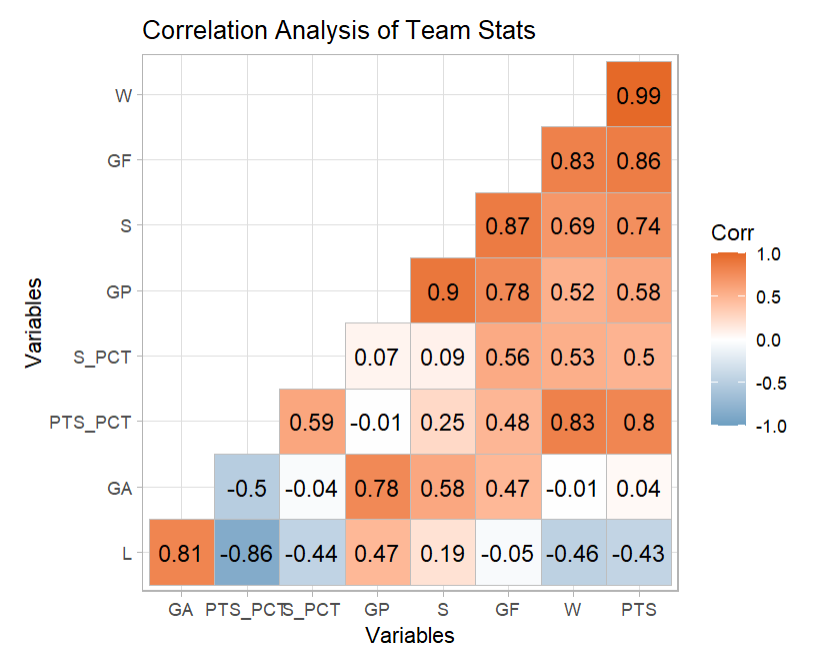
Two other interesting takeaways from this correlation analysis are:

• GF and W have a strong correlation at 0.86.
• S and W have a strong correlation at 0.74, yet S_PCT and W are at 0.5.

While correlation analyses don't tell the whole story, they help give you a high-level picture of the potential relationships within a dataset — ones that you can then explore more deeply in follow-on analyses such as predictive modeling.

To watch a quick-hit video tutorial, check out the YouTube video below.

Summary

Shot percentage is a fundamental hockey statistic that provides valuable insights into a team's offensive efficiency. Understanding its relationship with wins requires a multifaceted approach, including regression modeling, correlation analysis, and predictive modeling.

In this edition, we evaluated the relationship between shot percentage and wins using a simple linear regression model and a correlation analysis. We found that the relationship in both cases was similar to a flip of a coin. So, if you were to use shot percentage to try and predict wins, roughly half the time it would predict a win — and perhaps more distressing, half the time it wouldn't. We did discover other variables that appear to have a more positive relationship with wins, such as points and shots.

These analyses are a reminder that shot percentage, like other hockey stats, is just one piece of the puzzle. To gain a comprehensive understanding of a team's success, analysts must consider a multitude of factors, including defensive performance, shot quality, and game strategy.