How Successful is Our Power Play Strategy by Goals?

In this Edition

• Breaking Down the Question
• Structure of the Power Play Analysis
• Sourcing the Power Play Data
• Transforming and Summarizing the Data
• Creating the Power Play Analysis

Breaking Down the Question

Let's start by breaking down How Successful is our Power Play Strategy by Goals?

From the question, we can derive the following:

• How successful represents the scale for a metric that you will use to quantify the success of the power play
• Power Play Strategy is specific to the team, but represents the strategic space (e.g., plays employed during power plays, line combinations, etc.) against which you apply the metric
• by Goals is the metric that will be used to quantify power play success

Let's look at the structure of the power play analysis and then jump into a walkthrough.

Structure of the Power Play Analysis

We'll keep the analysis simple and evaluate the success of a power play and goals through the following:

1. Use the total number of power plays for a given team as the starting point. This represents the "surface area" of power plays within which a team may or may not score goals. You might also represent this through the percent of time on ice that a team is on the power play.
2. Calculate a small set of metrics, such as total number of goals scored, at the aggregate level (grouped by team) to measure the performance of a team on their power plays.
3. Create a calculated statistic that provides an overall performance metric for goals scored on the power play. This will be total goals scored per power play.

There are several ways to complete the analysis. We'll walk through different aspects of a hypothetically integrated system to show you different data management and analysis approaches.

To complete this analysis, we will:

• Source the data from a relational DBMS (SSMS) using SQL
• Transform, summarize and export the data using R and RStudio
• Analyze the data using Excel and Power BI

As you progress in your Analyst career, you'll understand how you can use R and RStudio, Excel and Power BI to directly query relational DBMSs and run the analyses within each of those tools or platforms, which will streamline much of the above.

Sourcing the Power Play Data

We downloaded the hockey data for this analysis from Kaggle. After downloading, we created a local relational database with data (across multiple NHL seasons). This process entailed:

• Creating a new database instance in SQL Express;
• Creating a data architecture for the tables (there is one with the download); and
• Importing the data from the CSV files.

Note that we had to tweak our data definition due to a few inconsistencies with the downloaded CSV files.

Once we had the database up and running and data imported into it, the tables looked as follows:

For this analysis, we didn't need all of the tables and data. To get the power play data, we used the game_skater_stats table. This table had all of the game and individual play data for each player and their team. Note that we also wanted the team name, so we used the JOIN statement on team_id with the team_info table and player_id with the player_info table. The SQL code to get this is below.

SELECT 
    gs.game_id, gs.player_id, gs.team_id, gs.pp_goals, gs.pp_goals, 
    gs.pp_assists, gs.even_time_on_ice, gs.pp_time_on_ice, 
    gs.time_on_ice, ti.team_name, pl.first_name, pl.last_name
FROM
    NHL_Hockey_DB.dbo.game_skater_stats AS gs
JOIN
    NHL_Hockey_DB.dbo.team_info AS ti
ON
    gs.team_id = ti.team_id
JOIN
    NHL_Hockey_DB.dbo.player_info AS pl
ON
    gs.player_id = pl.player_id;

Below is a snapshot of the results from the above query.

You can right-click the results and click Save Results As to save the query result to a CSV file.

Transforming and Summarizing the Data

With the data in a CSV file, you can now use it in your analytical tool of choice. You could go directly to Excel or Power BI if you want, but to illustrate how you can use R and RStudio, we took a stop there first.

Using RStudio, we first imported the CSV file, transformed the data and summarized it at the team level. For example, in the following code snippet you can see that we first imported the data into RStudio, added headers to the file, combined the FIRST_NAME and LAST_NAME elements to be PLAYER_NAME and then created a smaller dataset with fewer elements.

...
player_data_df = read.csv("player_level_pp_game_data.csv")

colnames(player_data_df) = c("GAME_ID", "PLAYER_ID", "TEAM_ID", "PP_GOALS", 
                             "PP_GOALS", "PP_ASSISTS", "PP_TIME_ON_ICE", 
                             "TIME_ON_ICE", "TEAM_NAME", "FIRST_NAME", 
                             "LAST_NAME") 

player_data_df$PLAYER_NAME = paste(player_data_df$FIRST_NAME, player_data_df$LAST_NAME, sep = " ")

sub_player_data_df = subset(player_data_df, select = c("GAME_ID", "TEAM_ID",
                                                       "TEAM_NAME", "PLAYER_ID", 
                                                       "PLAYER_NAME", 
                                                       "PP_GOALS", "PP_ASSISTS",
                                                       "PP_TIME_ON_ICE", "TIME_ON_ICE"))
...

We then summarized the data (using the dplyr library) at the team level. The following code illustrates how we did this.

...
library(dplyr)

team_pp_data <- sub_player_data_df %>%
  group_by(TEAM_NAME) %>%
  summarise(
    PP_GOALS = sum(PP_GOALS),
    PP_ASSISTS = sum(PP_ASSISTS),
    PP_TIME_ON_ICE = sum(PP_TIME_ON_ICE),
    TIME_ON_ICE = sum(TIME_ON_ICE)
  )
...

Note that beyond the above metrics we also created a metric called AVG_PP_GOALS, or the number of goals scored per power play. After adding this to the earlier data frame, the results of this dataset were an aggregated view using TEAM_NAME as the grouping element and a set of other metrics that we can use to evaluate the power play performance.

To export the data in RStudio, you use the write.csv() function (e.g., write.csv(df, "name_of_file.csv"), so we exported the above dataset to a local CSV file and how it was ready to use in Excel and Power BI.

Analyzing the Data using Excel and Power BI

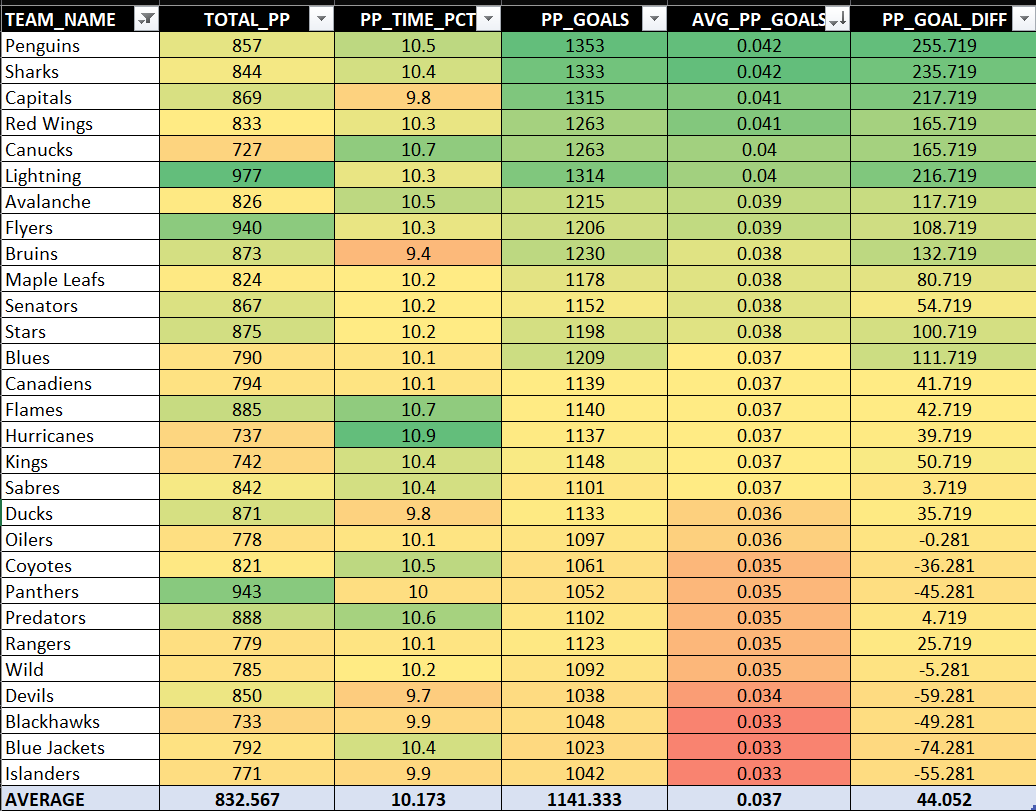
For the analyses, we kept it simple. In Excel, we opened the CSV file, formatted the data as a table and used conditional formatting. You can see the result below. Note that we sorted by AVG_PP_GOAL to show what team had the best goals per power play. It's a small margin with this metric to PP_GOALS (total goals scored on the power play) and PP_GOAL_DIFF (the difference of total goals scored from the average power play goals) give you more context on a team's power play performance through the lens of goals. Using conditional formatting, the heatmap gives you a good visual indication of which teams are doing better on the power play when it comes to goals.

Using Power BI, you can create a dashboard that auto refreshes when data is updated. (Power BI is really good for creating refreshable dashboards, and it has lots of data connectors so you can directly integrate your data with your dashboard.) For example, if you ran a daily refresh on the power play and goal metrics, you could have a fresh report each day. Further, if you're working for a specific team, you could have a league dashboard and then have subsequent team views that provide more dimensionality to the question of power play strategy – such as line combinations on the power play, team match-ups, and so on.

To create the Power BI dashboard, we completed three steps:

1. Created 'cards' for the Average Goal per PP, Average PP Goals and Average PP Percent of Time.
2. Plotted the PP Goal Differential (PP_GOAL_DIFF) using a column chart.
3. Created a table and added the teams, Total PPs, PP Time (%) and the total PP Goals.

The result was the following dashboard.

Some takeaways from this dashboard:

• Most teams are close to spending roughly 10% of their on-ice time on the power play.
• The average goals scored per power play is 0.04 goals.
• The average number of power play goals scored (across multiple seasons within the dataset) is 1,110 goals.
• The power play goal differential chart is interesting as it plots best to worst – the top three power play scoring teams being the Penguins, Sharks and Capitals.
• The heatmap table shows the Jets and Golden Knights as outliers because this was a multi-year dataset and the Golden Knights joined the league during this time and the Atlanta Thrashers moved to Winnipeg, so both of these teams didn't have the same level of historical data as the other teams. (We removed them from the goal differential chart given they were outliers and distended the visualization.)

When comparing Excel and Power BI, both have very powerful data processing and connection capabilities. Power BI is a more powerful as a platform for dashboards and has many different data connectors.

Check out the below YouTube video for a quick-hit walkthrough on how to use Microsoft Power BI to build the power play dashboard.

Summary

This power play analysis used game data from 2016 to 2019 (from Kaggle) as the source data. We then exported the data from SSMS (SQL Express) and then transformed and summarized the data in R/RStudio. We then exported the data from RStudio and created simple analyses in Excel and a dashboard in Power BI. The goal of this edition was to show you an analysis comprising multiple tools with different programming and platform capabilities. As a future Data Analyst/Data Scientist, you will leverage different tools and data modeling and analysis techniques.

Depending on your solution architecture, you can use RStudio, Excel or Power BI directly against a relational DBMS, so you don't need to export the data from SSMS (or your database of choice). You can also transform and analyze data using SQL or use scripting in Excel or Power BI to transform the data in either of those tools as well. Point being, if you are proficient in database programming with SQL and have a good front-end business intelligence (BI) tool, you can go a long way as a Data Analyst. As a Data Scientist/Sports Scientist, however, you will need to have more R and Python skills to build the deeper, more custom analyses and predictive models that are becoming the norm.

Subscribe to our newsletter to get the latest and greatest content on all things hockey analytics!