Final Predictive Model for the 4 Nations Face-Off Tournament

At a Glance

• Final Recap of the 4 Nations Face-Off Series
  Summarizing the multi-part newsletter series
• Process to Build the Predictive Model
  Lays out how we built the model to predict Goals per Game
• Building the Predictive Model
  Walks through correlation analysis and linear regression model
• Applying the Results of the Model
  Creates a final view of the match-ups using the predictive model

Final Recap of the 4 Nations Face-Off Series

This series explores the teams in the 4 Nations Face-Off tournament. The goal of the series was to explore the individual teams that are participating in the tournament with the end goal of predicting who would win the tournament.

Interestingly, our most popular quick-hit video of the series focused on Finland being the dark horse of the tournament.

To date, we've provided weekly predictions based on new learnings and analyses. You can check out the full series here. Today, we're going to nerd out and build a predictive model and then apply that model to forecast who will win each game in the tournament and potentially the overall tournament.

Across the series we've been pretty heavy on Canada winning the tournament, so let's see if our predictive model offers anything contradictory to that assessment.

Process to Build the Predictive Model

You build predictive models in different ways using a variety of techniques. And, for specific types of predictive use cases, you'll be bound to specific algorithms and approaches (e.g., linear regression for predicting values and logistic regression for classifying outcomes).

In this final newsletter, we're going to keep it simple and use a linear regression model to predict the Goals for each player in the tournament. We'll then adjust the Goals for the players, calculate the Goals per Game (GPG) per player, average the Goals at the country level and apply another adjustment for goaltending using each country's average Save Percentage (SP).

The process to build the linear regression model is as follows:

• Source the data to build the model;
• Conduct a correlation analysis to evaluate what hockey statistics most strongly correlate to Goals;
• Split the data into a training and test set and build the model using the strongest statistics;
• Apply the model to the 4 Nations Face-Off player data (which is a subset of the original dataset); and
• Adjust the model output and calculate the points gained/lost in each of the match-ups.

The result of the above will be a model that we can use to calculate the GPG for each team in the tournament, adjusted for the goaltending SP, that results in us forecasting who will win each match-up and subsequently which two teams go to the finals.

The tools we used to complete the above were RStudio and Microsoft Excel. We used RStudio to 1) clean and filter the data, 2) conduct a correlation analysis, 3) and build the linear regression model. We used Excel to build tables and reports that we could quickly create and export into PowerPoint for communicating the results of the model (in this article and our YouTube video).

Building the Predictive Model

When you explore the strength of the relationship among variables using a correlation analysis, you can test out many different variables. You'll want to be careful to consider the context of the variables, irrespective of strength.

For example, we selected the following statistics from our dataset, which showed positive correlations to Goals. Most of them also made sense. For example, you need to shoot to score, so higher shots on goal should result in goals (especially when we're talking about elite players) and more time spent on ice correlates to higher goals (you can't score when you're sitting on the bench).

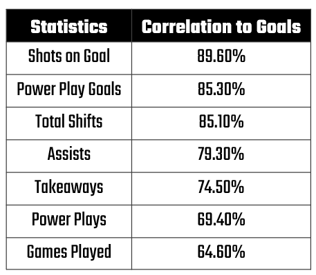
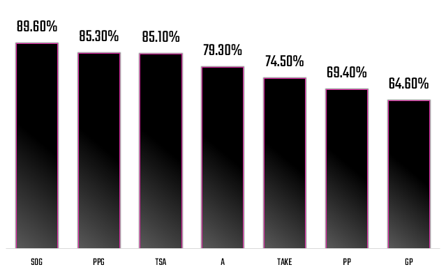
Here's a different view of the strength of the correlations, ranked strongest to weakest. Shots on Goal (SOG) clearly shows the strongest correlation in our dataset.

Now that we have a decent set of variables for the model, the next step is to create the Linear Regression model. We used one of the simpler approaches (the lm() function in R), which resulted in the following model.

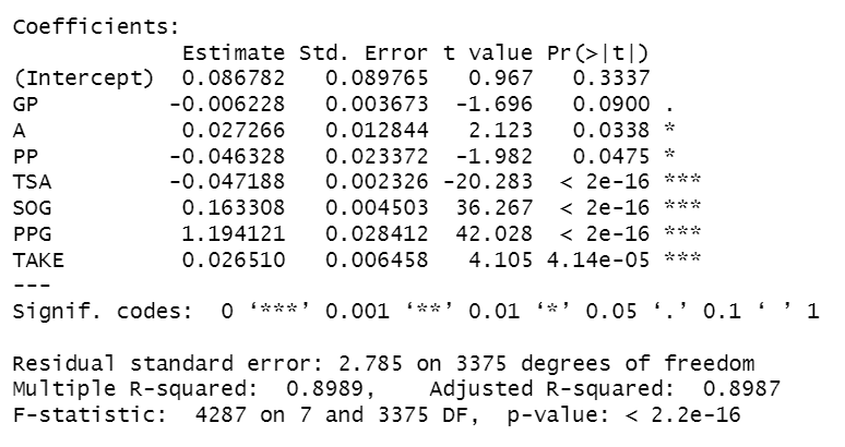
If this is Greek to you, a couple of key takeaways:

1. The variables are listed beneath Intercept, and the strength of the variable in the model is represented by the presence and number of asterisks.
2. Four variables are very strong (TSA, SOG, PPG and TAKE) and two are moderately strong (PP and A).
3. The level of significance is indicated by the p-values (which indicates the likelihood of obtaining a specific result in a statistical test). Statistically, you want to hit a p-value of 0.05 (95% significance) and even better is a p-value of 0.01 (99% significance).

Note that the significance of each of the predictors is strong (save for GP) and the overall R-squared value for the model is 89.9% – this is a good result.

At this point, you can use the model you've trained against a subset of the dataset to predict outcomes. This means applying the model to a test sample. One way to do this is cut the overall dataset into 80% training data and 20% test data and then evaluate the average delta between the actual goals and predicted goals in the resulting test. We would also recommend some degree of re-sampling here, so you don't just test the model once; keep testing it across random sub-samples.

After testing the test results, we also created a validation sample. Given our model is a very specific, one-off application of the model, our validation sample is made up from the players in the tournament. Here's a sample of the players, their representative country with the predicted GPG calculated from the model.

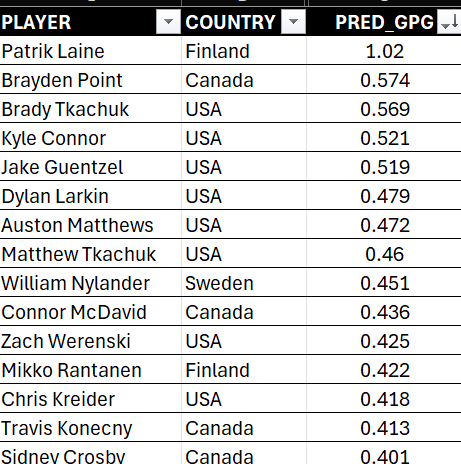
With the predicted GPG (PRED_GPG), we can then make other calculations using this value, which we'll explore next.

Applying the Results of the Model

So, here's where it can a bit wonky. With any model, you have to make assumptions, which could translate into statistical "corrections" or adjusted values. We made two adjustments to the GPG:

1. We adjusted for the quality of player in the tournament; and
2. We adjusted for the strength of the opposing goaltenders.

For the first adjustment, if we take each country and add the total possible GPG for each country, you get high numbers compared to the average goals scored in a hockey game (3.12 goals per game): 6.41 for the USA, 5.00 for Canada, 4.93 for Finland and 4.30 for Sweden. To account for the highly-skilled players, we adjusted the GPG down by 25%. This didn't change the ranking, but it does give us goal scoring closer to the average. Thus, the ADJUSTED GPG becomes the core GPG value to use in our prognostications.

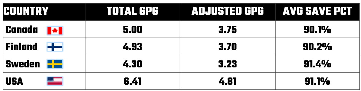
The second adjustment is the AVG SAVE PCT, which is used to further constrain potential goals against specific opponents. For example, when Canada plays Sweden, their ADJUSTED GPG is 3.75 * 90.2%, or 3.43. And you do this for each of the games to get an adjusted GPG that factors in opposing goaltending.

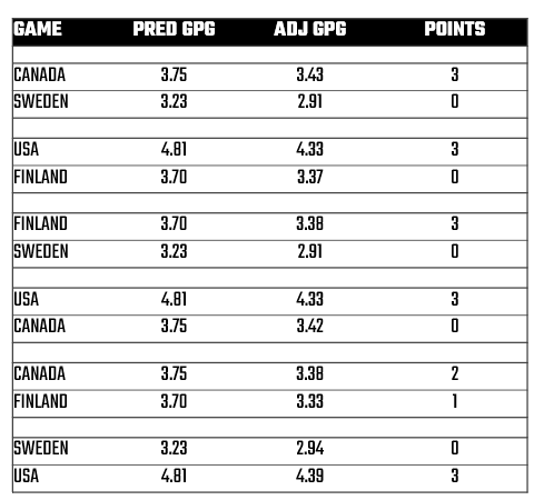
Now is this perfect? Hells no. But, for us armchair analysts trying to win the not-so-gentlemanly bet with our friends, this is better than no model at all. And the result for each game is below, where you see the teams in the game, the predicted GPG (PRED GPG) with the adjusted GPG (ADJ GPG) and the total points (POINTS) based on who has the higher ADJ GPG. (If it was close, then we assume overtime and revert back to our exploratory analyses for the final call.)

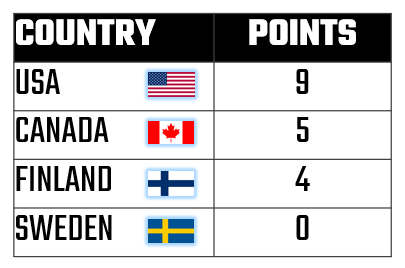
And if we tally the results of the above into the final Round-Robin tournament results, we get the following. So, using our model USA is the clear winner and it's a tight second between Canada and Finland.

Given the above, this means the final game of the tournament would be between the USA and Canada, and frankly it's a coin toss at that point. The teams have all played; they know one another's strengths; and all bets are off in the final game. And also remember: we didn't factor all of the possible correlations into the linear regression model, so there's wiggle room in the numbers.

Check out our quick-hit video for a high-level rundown on how to build and apply the predictive model.

All that said, it's interesting that there is directionality between the results above and the predictions we've provided over the last few weeks. That is:

• We vacillated between the USA and Canada as ranked top of the tournament. Here, the numbers bear out the USA as the top-ranked team.
• We saw Finland as the sleeper team and kept them at third. And there they are – in a pretty tight race with Canada.
• And sadly, Sweden is at the bottom.

Will the tournament have surprises? Yes. Will the tournament be laid out like the above? Maybe, maybe not. But, for those of you new to predictive modeling, this gives you an introductory look at how to build a simple model for a fun event that's right here in front of us. (Hopefully, it also shows you how complex predictive models can be, which is why a stable ML Ops and data pipeline are super important to tweak and test on a regular basis.)

Be sure to try out your own version of a predictive model to see how your algorithm will differ from ours!

Summary

In the 4 Nations Face-Off series, we explored each of the teams participating in the tournament to gauge their strengths and weaknesses. We did this from various dimensions such as offense, defense, grit, and goaltending. You can check out all of the newsletters here.

This was our final newsletter on the tournament, and we built a simple linear regression model to predict the final outcome of the tournament. Our model predicted the Goals at the player level, which we then adjusted by factoring in the skills of the player and the goaltending Save Percentage. We then used the resulting predicted GPG to forecast the outcome of each game and the assigned a point scoring to each game.

Whether the tournament bears out per our model is another thing altogether. But, it's going to be fun to watch!

Subscribe to our newsletter to get the latest and greatest content on all things hockey analytics!